In the last series of maps we are now doing a more indepth look at the German general election results. The following maps are all based on the second vote (Zweitstimme) and map these in various ways. To get a more precise view on what the majority of people decided for on the ballot, this time more than one party is mapped. This makes the maps more complex, but with the distinct colour scheme they remain understandable and show the results in a more differentiated manner. Click each map to get a closer view (in these maps quite important as colours might appear blurry in the shrinked maps shown on this page).
Except for the last two, all maps use the previously introduced population cartogram as their main projection, so that the proportions show the real population distribution.
On the first map, the largest parties in each constituency are included up to at least 50% of the votes. Usually these are the 1st and 2nd largest party – only few exceptions can be seen in the south, where CSU managed to get more than 50% of the votes in some areas:
Tag Archives: gridded cartogram
")
German election 2009 – Part II
Here comes a view on the first and second vote results: The two opposing maps show the party which got the most votes in a constituency, with he first vote (Erststimme) shown on the left and the second vote (Zweitstimme) on the right map (see the previous post or look here for more information on the German electoral system). Click the map for a larger view:

Both maps reveal the important role of CDU/CSU and (much less but still) SPD in the west, whereas DIE LINKE has this status in most of East Germany (including East Berlin). DIE LINKE’s dominance in the east is relativised by the lower population density in that part of Germany, as this projection reveals very well (see here for a conventional map of the election). In some constituencies in the west, SPD could manage to win a direct seat in parliament via the first vote, while the second vote went to CDU, mostly caused by strategic voters in favour of a more left politics and thus giving their first vote to the assumed more successful SPD candidate instead of their own favourite party.
However, further differences between the winners of first and second vote can not be seen from those maps.
The content on this page has been created by Benjamin Hennig. Please contact me for further details on the terms of use.
German election 2009 – Part I
From the previous posts you should now be quite familiar with Germany’s “new” shape when putting the population in perspective. If you are still struggling with it, try this map to see some important cities labelled on top of the map.
Let’s have a look at the results of the general election in Germany and start with the direct candidates elected to the new parliament. Due to the specific German voting system, each voter has two votes: one for a specific candidate in his constituency (and only one is elected per constituency), and a second vote for the party in favour. Those two votes can be for different parties. So the first vote reflects the MPs party affiliation for those elected directly to parliament.
And this is the map from the so called first vote (“Erststimme”) – click it for a larger view:

It can be seen, that FDP – the most likely new coalition partner of CDU/CSU – did not get any direct candidate elected at all, which is partly caused by the German electoral system that advantages the bigger parties for this vote (but balances this with the second vote).
But we wouldn’t need the map on the right side to see this. The map on the right side has much more interpretative value for those not familiar with the country’s structure: Pleasing for SPD supporters might be the effect of the high population density in the Ruhr-Area, blowing up the red patch in the west of Germany considerably and showing that there are still people left (!) to vote for their local SPD candidate. Pretty well shown is also the East-West division within Berlin, making the former Berlin Wall nowadays the border between DIE LINKE voters and the CDU/SPD part of the city (though SPD mostly is a matter of the suburban ring outside the western part of Berlin). Here our new map also shows clearly the only direct mandate of DIE GRUENEN – hardly recognizable on the conventional map.
There is much more to discover on this map…
The content on this page has been created by Benjamin Hennig. Please contact me for further details on the terms of use.
Germany’s Topography
While the polls are closed now, politicians are experiencing their personal highs and lows. But what about the population. What highs and lows are the people experiencing? Let’s now have a look at this as well. Here are an elevation map of Germany and a grid-based cartogram showing where and at which elevation most people are living at in Germany (click the image for a larger verson of the maps):

An improved and more detailed version of this map can be found here:
The Human Shape of Germany
The content on this page has been created by Benjamin Hennig. Please contact me for further details on the terms of use.
German constituencies and their population
Today is election day in Germany. So let’s have a closer look at the constituencies (Walbezirke) for this year’s general election – and how they actually look like in their real extent when showing their population size (click the image to see an even larger map):

The content on this page has been created by Benjamin Hennig. Please contact me for further details on the terms of use.
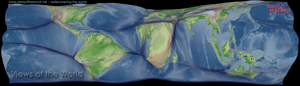
Re-Mapping the World’s Population
“Re-Mapping the World’s Population” – Presentation at the ESRI International User Conference in San Diego, 13-17 July 2009
Abstract:
The Worldmapper project has successfully produced a series of maps to visualize data, concerning a range of issues facing the modern world, based upon the idea of density-equalising maps. The Cartogram Geoprocessing Tool incorporating this density-equalising method has also recently been made available for ArcGIS. This presentation introduces and evaluates further new mapping approaches that move depictions beyond their simple descriptive form. It gives an insight into these new developments, focusing on sub-national level data which has until now been neglected. The world population cartogram demonstrates the first attempt to include sub-national density data. Within this approach, ArcGIS 9.3 plays a crucial role as an interface to convert suitable raster datasets and to produce updated cartograms. The data is converted using ArcMap’s Toolbox, while the Cartograms, due to their large size were, calculated in a Unix environment. The final visualization has been conducted in ArcMap.
(published 2009 in the ESRI User Conference Proceedings)

These are the slides from my talk:
The content on this page has been created by Benjamin Hennig. Please contact me for further details on the terms of use.